On one hand, the Kelly criterion is a basic math concept offering prosperity to those who understand it. On the other hand, it’s hardly included in any textbooks in economics, investing, or, for that matter, portfolio management. To my knowledge, the concept isn’t in the CFA program and I never encountered it during business school. Yet, the Kelly criterion is adopted by some of the most successful concentrated investors in the world, and the math behind it is irrefutable. Then why isn’t it more supported within academic circles?
The answer is two-fold: 1) it was invented by an information theorist, not an economist, and for that reason, economists reflexively defend their turf, and 2) there’s an over-emphasis on volatility-adjusted returns and widespread preaching of diversification in business schools. The Kelly criterion finds no place here because it doesn’t offer you a way to maximize your volatility-adjusted returns but instead offers you a way to maximize the growth rate of your wealth.
It’s interesting because the Kelly criterion was developed around the same time as modern portfolio theory. But while the Kelly criterion requires an estimate of the probability distribution of investment outcomes ahead of time, modern portfolio theory measures the risk of investments based on their past variances. This is why Markowitz’s mean-variance optimization is getting all the limelight. The Kelly criterion is too simple and suggests an inefficient market.
For any bottom-up investor, mean-variance optimization is a fool’s errand because the natural path of a bottom-up approach is toward a concentrated portfolio of mispriced securities. Yes, you can optimize through covariance between assets held in a concentrated portfolio to a degree, but you foremost want to make sure that the hard work you put into picking stocks will be well-rewarded through adequate position sizing so that your best bets reap the greatest returns. This is where the Kelly criterion dominates.
In this article, I explain how you should properly apply the Kelly criterion in value investing. But before that, there are two mental models to know before you can fully appreciate what the Kelly criterion has to offer and what it doesn’t have to offer.
So in the next section, I introduce the mental model of gambler’s ruin and the mental model of leverage. You may already think that you fully understand what leverage is, but perhaps you learn something new about how it affects wealth when it’s applied correctly and when it’s applied detrimentally over the long term and to sequential bets. The default thinking about leverage is in the short term. You’ll learn how to take a long-term view.
In the second section, I discuss how the Kelly criterion works. I then take what we’ve learned and apply that to the game of value investing focused on concentrated bets. I discuss the dangers that may come from naively trusting the Kelly criterion’s suggestions and propose a practical solution.
Gambler’s ruin
Professional betting — whether gambling, investing, or handicapping — is about having an advantage with a positive expected return. If you don’t have any statistical edge, you shouldn’t bet at all. But having a statistical edge is only one part of the equation; the other is the delicate issue of bet sizing (or “money management”). And I believe this other part is more delicate and critical than you think.
You can be the world’s greatest handicapper, but if you can’t manage your money, you’ll end up either broke or way below the potential of your hard work. The sad fact is that almost any gambler who has an edge but disregards money management goes broke in the long run.
This requires some explanation.
Let’s say you have an equal bet in which the odds of you winning or losing are 50% and the house takes nothing. You continuously bet a fixed dollar amount in each bet. In such a bet, the mathematical expectation of your wealth change is equal to zero. You are just as likely to win as you are to lose and the statistics say that your wealth should move in a horizontal line.
When we think about future expectations, we tend to rely on such statistics. But that’s pure fantasy. In reality, your wealth path would not move in a horizontal line. Instead, your wealth would follow a random walk that gets increasingly chaotic over time.
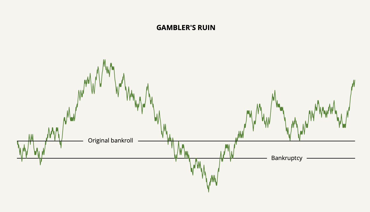
If we were to extend the wealth line into infinity, it would cross your original bankroll an infinite number of times. You would also go broke an infinite number of times. But this is irrelevant since you can only go broke once and then you’re out of the game. Notice how early bankruptcy happens.
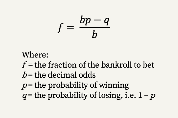
If you were to play a negative expected-return game such as in a casino, the path to bankruptcy would happen even faster. And even if we were to give a small statistical edge such as a 51% win rate, it’s still possible for a persistent gambler to go broke at some point. This is the gambler’s ruin problem.
Knowing this, consider now the foolish betting strategy by the name of martingale. This is the strategy in which you double your bet every time you lose until you win. The effect of the martingale system is that it accelerates the gambler’s ruin problem.
The solution to gambler’s ruin, as I think you’ve already figured out, is to bet bankroll proportions instead of fixed dollar amounts so that you bet more as your bankroll increases and you bet less as your bankroll decreases. But even doing that doesn’t shield you from gambler’s ruin if your betting proportions are too aggressive for your statistical edge.
So now the question becomes: how much of the bankroll should you bet? Is there an optimal bet size that assures you to never fall prey to gambler’s ruin while maximizing your long-term wealth?
Leverage
Leverage has counteracting forces: It either amplifies your gain or amplifies your loss. Almost everyone understands that. But not everyone understands how these counteracting forces come into play when applied over longer periods and through multiple bets, even as these bets have positive expected returns.
Say you have a rigged coin-tossing game where the coin is designed so that it lands on heads 51% of the time and lands on tails 49% of the time. The payoff is even. You are well aware of the coin’s design and you know that the probabilities are in your favor. You now also know that you must bet bankroll proportions to avoid gambler’s ruin.
Let’s first see what might happen to your wealth over time if you continuously bet 1%, 2%, or 5% of your bankroll on heads 1,000 times.
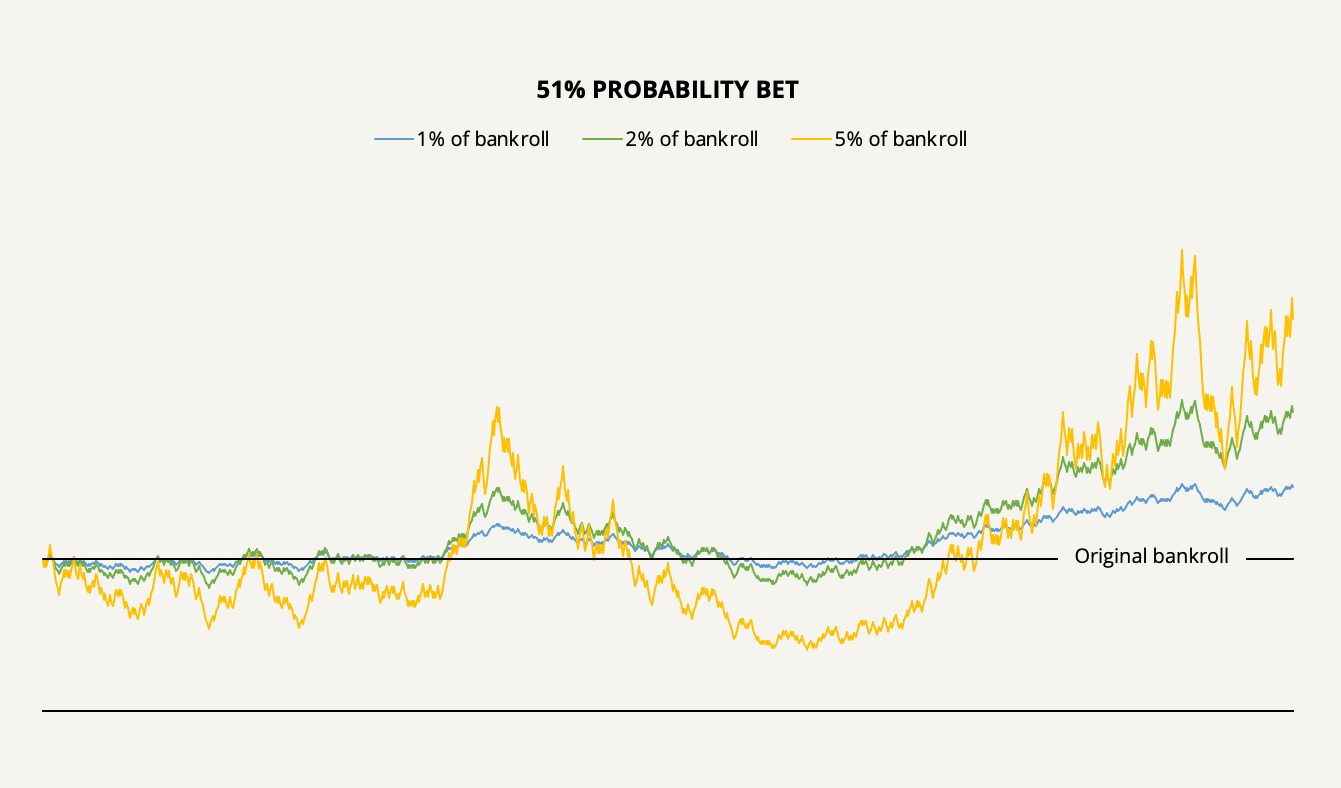
With a 1% betting strategy, the simulation shows you could have made a 47.7% return on your original bankroll with mild volatility. You could also have made a higher return, albeit more volatile, with larger bet sizes. This is the intuitive way to think about leverage.
Now, let’s look at the counter-intuitive reality of what happens when we increase your bet size even more, say to 10%, 15%, or 30% of the bankroll with each bet.
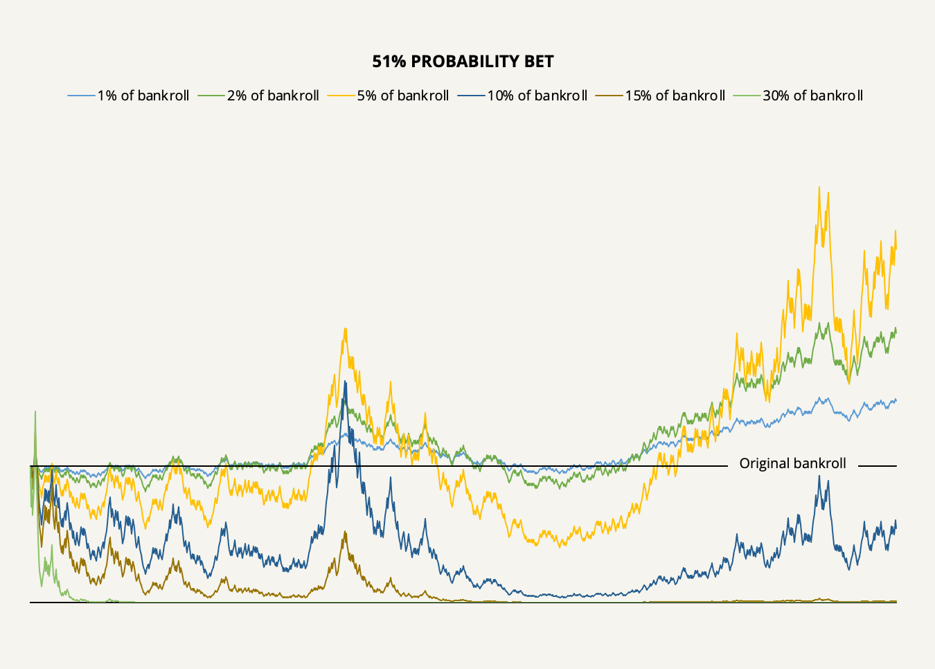
As our simulation shows, it’s easy to lose money, even with a mathematical advantage. Increasing your bet sizes too much will devastate your bankroll: with a 10% betting strategy, you’d only have half of your bankroll left, and with 15% and 30%, your bankroll would essentially be ruined.
Think about what’s going on for a minute. With a 5% bet size or 2% bet size (which, as we’ll later find, is the long-run optimal), your bankroll would increase faster than a 1% bet size. But with a 30% bet size, it would lead to fast ruin. In the first case, leverage is helping, and in the second case, it’s detrimental.
Why is that?
The reason is that at a very specific point, the marginal profit you earn from adding more leverage shrinks and eventually turns negative. To further explain, let’s switch our example around to an equal probability bet but with unequal payoffs which requires actual leverage in the terms of borrowed money.
Say you have an investment opportunity that is 50% likely to work out. If it does, you will earn a 20% return on your investment, and if it doesn’t, you will lose 10% of your investment. The payoff ratio is therefore 2:1 and the reason why we can now borrow money to amplify our return is because risking 100% of our capital can only lead to a loss of 10%.
Now, instead of doing a 1,000-bet simulation, let’s only do two successive bets: one win and one loss (the order doesn’t matter). Then we can iterate using different levels of leverage.
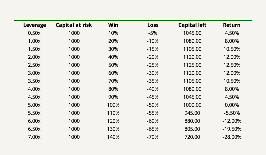
What we see is that as soon as the leverage exceeds 2.5x, the return made from the two bets starts to drop off and eventually goes negative at >5x leverage.
The reason why this happens is that the loss incurred on the second bet more than offsets the return made on the first since that loss is taken from a larger pool of capital. It’s the same geometric effect as if you gain 10% on an investment and then lose 10%, you’re one percent down on your original investment.
It’s when this marginal geometric effect exactly offsets the marginal benefit of adding more leverage that you have the optimal level of leverage. In this case, the leverage that maximizes your return is 2.5x.
Now that we understand the mental models of gambler’s ruin and leverage, we are ready to move on to the Kelly criterion.
The Kelly criterion explained
The beautifully simple formula for the Kelly criterion calculates the optimal proportion of your bankroll to bet to maximize the geometric growth rate of your wealth. But not only does it promise you maximum profit from effectively leveraging your opportunities, it also promises you safety from gambler’s ruin.
f is the proportion of your bankroll that you should bet which is the function of the probability of winning, the probability of losing, and the odds you have — i.e. the payoff ratio.
The Kelly criterion has three prerequisites:
- You must know the exact odds and probabilities to input.
- If only one of them is in your favor, it must more than offset the other, i.e. there must be a positive expected return.
- You must scale the Kelly output so that the amount you bet is equal to the potential loss.
The last point is vital and it’s where I see lots go wrong when using the formula. Many websites don’t scale the output correctly when dealing with a situation where you can lose “some” but not all. It’s amazing how far up the academic ladder this goes. Seeing how so many practitioners of the Kelly criterion get this wrong brings home a quote of Ed Thorp’s from his early days in the stock market that he was both surprised and encouraged at how little was known by so many.
The Kelly criterion must be used in such a way that what is bet must equal the potential loss. It’s inherent in the word “bet”: What we bet is what we put on the line. In our leveraged investment example, the base loss was 10%, so if we were to put 100% of our capital into the bet, we could only lose 10%. Thus, the right thing to do in this case is to scale the output by 10 which leads to a leveraged bet.
Let’s take our examples so far and put them into the Kelly formula.
In the rigged coin-tossing game we had a 51% win probability with equal payoffs. Inserting these inputs in the Kelly criterion formula shows that the optimal betting proportion of our bankroll is 2%.
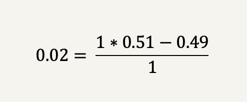
In our investment example, we had a 50% win probability with unequal payoffs of 2-for-1 (20% win vs. -10% loss). The Kelly criterion, therefore, suggests betting with a maximum loss of 25% of the bankroll which, as we found out, is equal to a 2.5x leverage from the base loss of 10%.
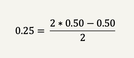
Let’s take a more normal investment example that wouldn’t require leverage in the terms of borrowed money. Say you found a company that you believe is worth at least $100/sh and it’s currently trading at $80/sh. You’re only 50% certain that the company is worth your intrinsic value estimate.
The odds in this case is 1.25 (100 divided by 80) and the Kelly criterion thus suggests to bet 10% of the bankroll on the investment.
It all looks plain and simple. But what if we dive a bit more into the engine?
Think about the fact that the Kelly criterion promises you maximum profit while protecting you from ruin. Such promises may sound antithetical. But the root idea behind the Kelly criterion is that there is a tradeoff between risk and return which we can present as the Kelly curve.
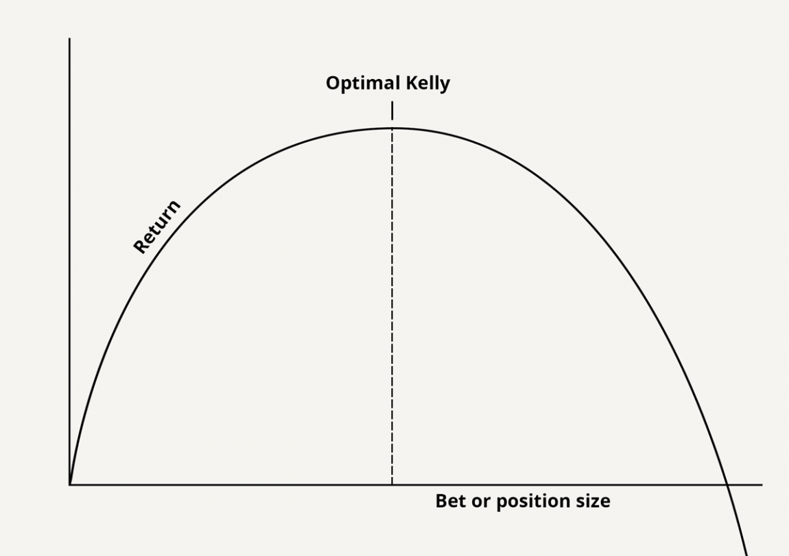
Notice two things:
1) Notice how near the top the increased return you get from adding extra risk becomes tiny. In fact, as the bet size approaches the top, the ratio of marginal risk to marginal profit goes to infinity. Eventually, you’d have to risk an additional $1bn to earn one more cent of expected profit. The reason is that the Kelly criterion assumes no value is placed on risk as long as it maximizes the return.
2) Notice that betting just a tiny bit more than the Kelly criterion suggests leads to decreased profits with higher risk (which we already know from the mental model of leverage).
This means that the goal is not necessarily to pick the exact top of the Kelly curve. The goal is to stay within the left side. The left side represents rationality while the right side represents irrationality, or insanity.
Let’s see what might happen if we were to underbet or overbet the Kelly criterion’s suggestion using our unequal payoff example in a 100-bet simulation.

Consistent with the two-bet example, the Kelly-optimal betting size, of course, leads to a significantly higher return in the long run as compared to underbetting or overbetting. The longer we stretch out the time horizon, the bigger this difference is going to get by compound interest.
Does this mean that we should always try and stretch for the Kelly optimal point as long as we’re on the left side of the curve? No, it doesn’t. In the vast majority of cases, especially in investing, it makes sense to err on the side of caution and underbetting may be the right strategy in the long run. To understand why that is, we can now introduce another mental model: the law of large numbers.
The Kelly criterion applied to value investing
There is one oft-overlooked catch to investing: life is short and opportunities don’t come around often. In games such as our coin-tossing example, you could either double or lose your bet every few seconds. In investing, doubling your money takes years.
The problem is that this nature of investing goes against the engine behind the Kelly criterion: the law of large numbers. Ever since it was proved by Jakob Bernoulli in 1713, this law has caused a lot of confusion of gamblers (and investors).
In roulette, there’s an 18/38 chance that the ball lands on red in any game played. But if you were to play the game of roulette 38 times in a row, you, of course, wouldn’t expect the ball to land on red exactly 18 times. Likewise, if you were to play the game 38mn times, you’d in no way expect it to land on red 18mn times. No matter how many times you play, there’s never any certainty of achieving the expected number of reds. But as the number of games is increased you can expect one thing: that the % of reds landed will tend to come closer to the expected percentage. This is the law of large numbers.
Investing isn’t a casino game and you won’t have many sequential bets. Therefore, absent a certain fulfillment of the law of large numbers, the Kelly criterion may involve more short-term risk than you might be prepared to take.
This has another effect: You can only pick the opportunities in which you have a significant edge. A winning probability of 51% in a coin-tossing game isn’t worth much if you can only bet once. Of course, the natural effect of this is towards a concentrated portfolio.
But how concentrated?
It depends on your ability to estimate probabilities and correctly value companies. The stock market is not a controlled environment where odds are static and given in advance. The odds are fluid, they change daily, and it’s difficult to get enough of an edge to make a bet.
I propose a four-fold solution to these problems:
- Be conservative in your intrinsic value estimate (which determines your odds) and your level of confidence in the estimate (which determines your probability).
- Apply at least a 20% margin of safety to the Kelly criterion’s suggestion.
- Invest only in companies where there’s at least a 70% probability of you being right in your valuation.
- Treat the Kelly criterion as a thought experiment rather than a mechanical exercise.
The first point mitigates the fact that in valuing companies, overconfidence is almost always a factor, and reality will almost always turn out less profitable than expected.
The second point provides an appealing trade-off. Only betting fractions of the Kelly criterion limits the probability of drawdowns by an exponential factor. For example, when you apply a 50% margin of safety (only betting half of the Kelly criterion’s suggestion), you end up with 75% of the optimal profit while your risk is reduced by half.
The third point ensures that you keep within your circle of competence, which is the most important point in this entire discussion.
And lastly, the fourth point urges you not to try and calculate the Kelly criterion’s suggestion for everything. Trying to pin down an exact position size can blind you from the dynamic nature of investing and valuation. When your edge is large enough, you will know to bet big.